In understanding my approach towards creating SkyTools 4 Imaging, its worth considering how major professional observatories, such as ESO, use mathematical models of their telescope and instruments to plan their observations. It is useful to know the image scale, what exposure times to use, whether a star will bloom or if the signal will become nonlinear, and how many exposures are required to reach a given Signal to Noise Ratio (SNR).
I have long thought that amateurs could greatly benefit from such a tool, but many of the difficulties in doing so seemed insurmountable. The professional apps tend to focus on one telescope, one instrument, and a specific type of work such as spectroscopy. To be truly useful to the amateur, an app would have to work with any telescope, camera, and filter. Most difficult of all, it would have to handle a range of target objects such as stars, galaxies, and emission nebulae.
My previous software product, SkyTools 3, is primarily aimed at visual observers. It does have an imaging capability, but it uses a crude imaging model that suffers from many shortcomings. The model was originally developed by Bradly Schaeffer and it makes many simplifying assumptions, such as filters that must be approximately Gaussian, and it has no means of handling emission line objects, such as HII regions and supernovae.
It was a first step, but only that. In order to be more useful, I would need a much better model, and I would have to invent ways to approximate both the spatial and spectral energy distribution of everything from comets to planetary nebulae.
In the end, SkyTools 4 Imaging took over four years of full-time work and introduces an entirely new imaging system model. It begins with the target object and ends with an accurate prediction of the target object signal, sky signal, system noise, and finally SNR. Any set of observing conditions can be simulated, including the effects of seeing, airmass, twilight, and moonlight.
So how does it do it?
Spectral-Energy Distribution of the Target Object
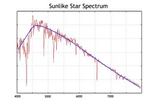
Stars and other stellar sources (quasars, minor planets, etc.) are modeled based on the continuum, which can be described by their UBVRI color indices (see Figure 1).
Reflection nebulae, galaxies, and comets are modeled similarly, using UBVRI colors representative of these objects. For galaxies, the type of galaxy determines the color characteristics.
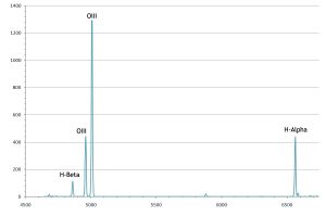
Planetary nebulae, HII regions and supernova remnants are modeled via their emission line spectrum (see Figure 2). The primary emission lines used in SkyTools are H-Alpha, H-Beta, OIII, NII, and SII. Other lines are included when data is available.
For some objects, (HII regions and supernova remnants in particular) there is no catalog data available for the required emission line strengths. To obtain data for these objects I have scoured the scientific literature. For those that remained without sufficient data I have initiated an observing campaign using narrow band filters to measure the emission.
Atmosphere
For a given object, the total energy as well as the energy distribution is modified as it passes through the atmosphere. The degree to which it is modified depends on the airmass, atmospheric conditions (temperature, humidity), and time of year.
The brightness of the sky background depends on the amount of light pollution, moonlight, twilight, altitude of the target, and atmospheric conditions.
Telescope Optics
The area of the telescope objective, minus what may be obstructed by the presence of a secondary mirror, determines how much total energy is collected. The optics also modify the spectral distribution, depending on the optical coatings. In the case of reflecting optics, the time since the mirror was last cleaned has a significant effect.
Filter
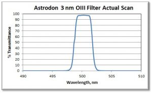
A filter is modeled by combining the spectral transmission curve of the filter with the energy distribution of the target object, as modified by the atmosphere and optical system (see Figure 3).
Camera Detector
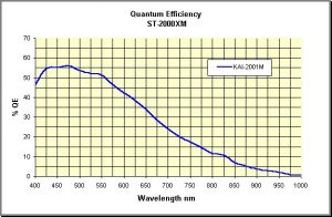
At the final step, the number of photons counted by each pixel is the integral over wavelength of the spectral energy distribution of the light that reaches the detector, combined with the spectral quantum efficiency of the detector. The quantum efficiency tells us how many electrons are produced for each photon detected (see Figure 4).
As a result of the previously mentioned steps, the signal in e- (electrons) can be predicted. For extended objects it is predicted on a per pixel basis, along with the signal from the sky background. The signal measured by each pixel in e- is converted to ADU via the camera gain. The SNR can be estimated per pixel based on the signal and the total noise (primarily composed of detector readout noise and sky noise).
For stellar objects the total signal in e- is predicted. The atmospheric conditions and limitations of the telescope optics determine how this signal is spread over the detector, as modeled by a point spread function. The photometric SNR is computed for the total signal and noise over a circular aperture. The peak SNR is computed for the peak signal (peak of the point spread function) and the estimated noise at the peak.
Diffuse objects such as galaxies, nebulae, and comets, are not uniform. For example, a spiral galaxy may consist of a bright central core, spiral arms, and a faint outer halo.
So, when estimating the SNR, it is important to specify what part of the galaxy we are exposing for. Do you wish to merely detect the bright core? Or do you wish to obtain a high-quality (high SNR) image of the spiral arms? The surface brightness corresponding to each part of the galaxy is estimated by a combination of the overall brightness of the galaxy and statistics for galaxy type.
A similar process is used for other diffuse objects, such as reflection nebulae. For comets, the size of the coma and degree of concentration from recent observations are used.
Testing
The model has been tested extensively using the many imaging systems available at iTelescope.net.
The primary testing was done with Landolt UBVRI standard star fields. I developed an image analysis app that uses the information from the FITS header along with photometry extracted from the image data. The photometry was tested against software from the AAVSO to ensure its accuracy. For each image the actual signal is compared to the signal predicted by the model for the time and conditions of the image.
Interestingly, several additional significant effects were uncovered in testing, such as the age and cleanliness of the mirrors, and the optical transmission of the camera window.
In the end we can compute the SNR for any exposure at any time during the night. But what if the conditions are changing rapidly? E.g. what if the sky brightness is changing during the exposure? Or for an image of a comet at high airmass, the airmass can change quickly as it sets.
Standard SNR calculators implicitly assume that conditions don’t change during the exposure. But the SkyTools Imaging calculator integrates the signal, sky brightness, and other factors, over time. As a result, it can estimate the SNR of an image even when the conditions are changing rapidly during the exposure.
Finally, we can create a model with real world inputs that are based on the properties of the target object, location, weather conditions, airmass, sky brightness, and imaging system. This can be very useful by itself, but we can take it a step further. For any time of night the SNR can be computed for an arbitrary exposure. We can also compute the SNR for the same exposure, but under the ideal conditions at the same location. When we compare the two by dividing the SNR computed for the test exposure by the SNR under ideal conditions, we have an index that can be used to estimate the imaging quality (IQ) at any time. This is extremely useful for planning when to image in each filter.
Conclusion
It has been a long journey, and I faced many apparently insurmountable problems, but I am very happy with the result. I can’t imagine planning my own imaging without it. I use SkyTools 4 Imaging to select targets that are appropriate for an imaging system, determine the number of exposures and sub exposure times required to meet a target SNR, maximize my SNR by planning my images during the best time of the night, and even to select which available telescope is best for a given target.
 Greg Crinklaw operates Skyhound and is the developer of SkyTools. He is a life-long amateur astronomer, who is also trained as a professional astronomer, holding a BS, MS in astronomy, and an MS in astrophysics. He also worked for NASA as a Software Engineer on a Mars orbital mission. Greg and his family live in the mountains of Cloudcroft, New Mexico.
And to make it easier for you to get the most extensive telescope and amateur astronomy related news, articles and reviews that are only available in the magazine pages of Astronomy Technology Today, we are offering a 1 year subscription for only $6! Or, for an even better deal, we are offering 2 years for only $9. Click here to get these deals which only will be available for a very limited time. You can also check out a free sample issue here.