Editor’s Note: To show the MiniWASP Parallel Imaging Telescope Array images in greater detail, they are included at the end of the article in large format. To view hi-res images of the ones included in this article and others visit New Forest Observatory.
Astronomy Technology Today recently chronicled one man’s struggles in getting a two-imager system up and running, which prompted me to put this article together. Here, I outline the development of the MiniWASP Parallel Imaging Array, a highly flexible five-imager parallel imaging array for deep-sky imaging.
A Bit of Backstory
My adventures in deep-sky imaging began in the Autumn of 2004 when I managed to achieve first-light with an (original) HyperStar and a Celestron NexStar 11 GPS Schmidt-Cassegrain Telescope (SCT). As this was my very first foray into deep-sky imaging, I had no idea, at the time, just what an extremely powerful imaging system I had put together. I was also completely dumbfounded why everybody wasn’t imaging with the HyperStar, as it made life so easy.
The HyperStar is a x1 corrector that allows you to place your imaging camera at the prime focus of an SCT, that is, in place of the secondary mirror. So, what the Hyperstar does, extremely effectively I might add, is to flatten the highly curved wavefront that comes up to the imaging camera from the primary mirror. So, the Hyperstar basically turns the native f/10 SCT into an extremely fast f/1.8 Schmidt-camera.
In the old days of photographic film, where film was placed at the prime focus of a Schmidt-camera, the film would be firmly attached to a curved back-plate to compensate for the curved wavefront from the primary mirror. Since it is impractical to fabricate CCD cameras with a curved sensor, it was necessary to find an optical solution to flattening the curved wavefront, and that solution was the highly effective HyperStar lens assembly.
I won’t go into the details of the problems of imaging with the original HyperStar, which didn’t have collimation adjusters or camera rotation adjusters, as these are discussed in an earlier ATT article (Volume 2, Issue10, 2008). However, I will briefly describe imaging with the system using a tiny Starlight Xpress H9C one-shot colour (OSC) CCD camera.
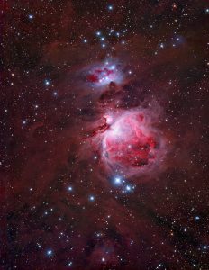
For the original Hyperstar, the H9C was about the right physical size of sensor to ensure no vignetting. It is a tiny chip by today’s standards – only 9 x 6.75 mm in size and only 1.5 Megapixels – but it performed superbly well with the original f/1.8 HyperStar. And at f/1.8, it meant of course that sub-exposure times could be extremely short (I used a maximum of just two-minutes in those early days), which meant impressively round stars and glass-smooth images resulting from stacking together the typical 100 sub-exposures I used to employ. Figures 1, 2 and 3 show typical results from the f/1.8 HyperStar/C11 combination.
As you can see, the quality of the images from the H9C/C11 combination is pretty impressive, provided focus and collimation are spot on.
The only negative aspect of imaging with this kit is the very small field of view (FOV), and I have always been much more interested in “the bigger picture.” Starlight Xpress then came out with a 6-megapixel OSC CCD they named the M25C with an APS-size chip (basically half the size of a 35-mm frame), and I just had to have one of these. Unfortunately, I could not put one onto the original HyperStar, as it would have produced terrible vignetting. So together with the M25C, I bought a Takahashi Sky 90 refractor with the reducer/corrector lens giving me f/4.5 imaging at a focal length of 405 mm and a focal plane diameter that covered the M25C sensor nicely. This arrangement was piggy-backed on the C11, which of course meant that my beautiful C11 was now relegated to the role of guide-scope – not a very satisfactory solution.
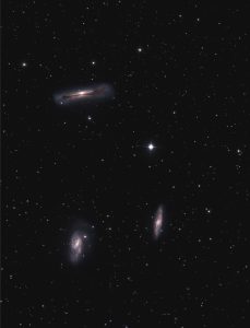
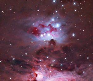
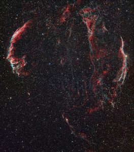
I had a great year imaging with the Sky90/M25C combo, and the massive 3.33- by 2.22-degree field of view was just what I was after. However, at f/4.5, the Sky 90 was a massive 6.25-times slower than the HyperStar for extended objects (nebulae), and this really showed up in the (now) extremely long total integration times I had to suffer to get a good quality image. So, by the end of the first year of imaging with this kit, I was extremely happy with the size and quality of the images produced, but I was becoming very frustrated at the length of time it was taking to capture these images, especially in the U.K., where clear, Moonless nights are few and far between. This also meant that my output, in terms of numbers of deep-sky objects captured per year, crashed. Figures 4, 5 and 6 show typical images from the Sky 90/M25C combo. You can go deep, but it costs you a lot of time.
You can see that it is possible to get decent-quality images of the brighter nebulae from this kit, but there is an enormous time penalty to be paid. It took a whole summer’s worth of good imaging nights to get the Veil nebula done properly, and by then the novelty of the nice wide-field had worn off. I was really missing the speed of the HyperStar.
I will admit that, at this point in my imaging, I became a bit despondent; the Sky 90/M25C was giving me the FOV I wanted at the cost of enormous amounts of integration time, and the original HyperStar gave me the speed I wanted but at the cost of a much smaller field of view. I really didn’t know what to do next. And then, as luck would have it, at exactly this point in time, Starizona came out with the HyperStar 3.
The HyperStar 3 is an f/2.0 corrector with several major upgrades on the original f/1.8 HyperStar. For me, the most important improvement was the larger focal plane diameter, the new HyperStar 3 could be used with the larger M25C CCD. But the HyperStar 3 also came with collimation and camera angle adjusters, so now it was also possible to perfectly collimate the new version before an imaging run. Collimation, and how you achieved it, was always a major issue for the original HyperStar.
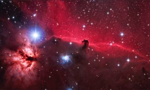
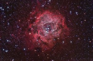
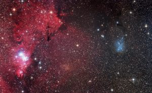
Hooray! I was back in business – the HyperStar was back at the New Forest Observatory, and all was fun again … for a while at least. Figures 7, 8 and 9 show work carried out with the HyperStar 3 and M25C OSC CCD.
Well, I now have the field of view I want, at the speed I want, so what could possibly be a problem now? I had two issues with the kit. First, I couldn’t take single-star images of the bright constellation stars, something I like very much as an imaging subject. Why? Because all that glass in the HyperStar 3 creates large ghost flares from the brightest stars, even with the lens edges blackened. The Sky 90 causes no – zero, zilch – ghost imaging, even from the brightest star in the sky, Sirius, so the Sky 90 still had that advantage over the HyperStar 3.
There was in addition an indefinable quality to the star images in the Sky 90 that I found lacking in the HyperStar 3 images – I really can’t tell you what it is; maybe it has something to do with the improved contrast of a refractor – but that “quality” I found was missing in the HyperStar 3 images, and so I found myself once again at a crossroads in deciding how I am to go forward in my imaging.
This latest decision point also came at a very convenient time. I was fast approaching September 2010, and I would be taking early retirement from my job as Professor of Photonics at the University of Southampton. I needed to get a mega retirement project sorted out!
A Mini-WASP Solution
This is a good time to summarise the situation to see a possible route forward. I had the HyperStar 3 on the C11 with an M25C OSC CCD. This was the perfect imaging rig for faint objects and nebulae at a reasonable FOV. Its only real downside is the inability to image the brightest stars. I had the Sky 90, which was perfect for the brightest stars and star fields, but was no good (time wise) for nebulae and fainter objects. It was at this point that I thought about the SuperWASP (www.superwasp.org ) arrays for exo-planet hunting.
These arrays use eight or more DSLR lenses to cover very large FOVs during an imaging session. For the Super http://www.superwasp.org/index.htmlWASP array, the FOVs of the individual lenses are made to overlay so that a mosaic can be put together very easily. My idea was to copy the SuperWASP layout and to use several Sky 90s imaging in parallel, but all imaging the same object (total overlap).
Why do this? If we have, say, N Sky 90s, then in one-hour of imaging time we get down N-hours’ worth of data, so we can cut down the very long integration times by a factor of N. We also get the ability to image the brightest stars without ghost flaring and that “indefinable” quality thrown in for good measure. So that’s the retirement project sorted out – I would put together my own MiniWASP array using Sky 90 refractors and the new M26C 10-Megapixel OSC CCD cameras from Starlight Xpress.
A Mount and Observatory for the MiniWASP Parallel Imaging Telescope Array
The first thing to consider was the mount. All that kit was going to weigh a lot, and at the time there were only a few mounts on the market to consider. Of those, I chose the Paramount ME. Having always worked with an alt-az mount on a wedge, I didn’t know what I was letting myself in for, but just let me say that, although the Paramount ME does its job to perfection, I just hate GEMs.
For the sort of work I wanted to do, an alt-az on a wedge is far more useful and convenient, but a Paramount ME it had to be. I then drew up a suitable frame to hold four telescopes rigidly in place and got a local engineering company to make it for me in aluminium.
I needed to buy a second Pulsar fibreglass dome to house the MiniWASP Parallel Imaging Array as I wanted to be able to run the HyperStar as well as the MiniWASP, and I also had to buy several computers as the easiest way to run the multi-imager system was to have one computer per camera. An imaging friend, Tom How, who is a software and electronics expert, built me an automatic dome rotator for the Pulsar dome, which keeps the dome aperture nicely placed in front of the array, wherever the array is facing (and as it is tracking of course). Tom also sorted out the software to synchronise the three CCD cameras, so that they would all start at the same time for each sub-exposure with dithering enabled. This was not a trivial job!
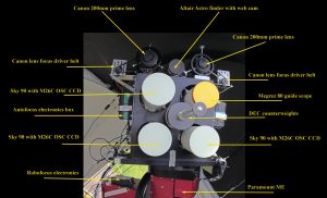
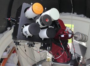
The main aluminium frame has four openings for four telescopes. Three of the telescopes are Sky 90 imagers, and the fourth scope is for a Megrez 80, which is used as a guide scope. It would have been possible to fit an off-axis guider and have a fourth Sky 90 as an imager, but I have heard of the issues in trying to find a guide star (sometimes) using that approach, and I simply didn’t want that sort of frustration on a clear Moonless night, so I stuck with what I know. To date, I have never had an issue with finding a guide star with the separate guide scope and Lodestar guide camera. Figure 10 shows the MiniWASP Parallel Imaging Array optical head, with a few more bits on the top plate that we’ll come to later.
Imaging with the MiniWASP Parallel Imaging Telescope Array
It was time consuming, but fairly straightforward to set up the array for imaging. I chose one of the Sky 90s as the “master” and then aligned the other three scopes to point at exactly the same place as the master scope. With the MiniWASP Parallel Imaging Array, each scope is held in place in the same way that scopes are held in standard guide-scope rings so I can easily move the individual scopes within their respective circular cut-outs using six adjuster bolts with nylon heads. There is no need for any lock nuts on the adjuster bolts, as I found no “flexure” in the array, even with hour-long sub-exposures.
So, we’re all set and ready to go with the array, and it’s time to see what it can deliver. Figures 11, 12, 13, 14, 15 and 16 give you an idea of the power and the flexibility of this parallel imaging system.
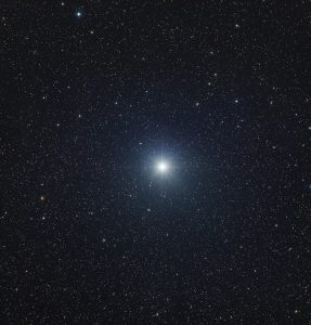
An acid test for imaging a bright star is to pick the brightest star in the sky – Figure 11 shows Sirius. This is a vertical two-frame mosaic using two-minute sub-exposures and an actual imaging time of one-hour per frame, making a total integration time of three-hours per frame.
In Figure 12, we see Polaris and a hint of the Integrated Flux Nebula (IFN). These sub-exposures are only five-minutes long as guiding is turned off when imaging near the Pole. However, eight-hours of total integration time is sufficient to start showing the IFN quite nicely.
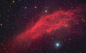
Figure 13 shows how the Sky 90 array copes with nebulae. This is around 16-hours’ worth of integration time, including 20 and 30-minute subs on the California nebula.
In Figure 14, we see the Pleiades using around nine-hours of 15-minute subs and a further nine-hours of 40-minute subs. It took the 40-minute sub-exposure to show up the very faint dust seen along the bottom left edge of the image.
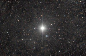
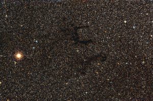
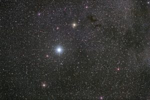
Figure 15 shows Tarazed and Barnard’s “E.” This is a combination of around nine-hours of 10-minute subs and a further nine-hours of 20-minute subs. Remember that the nine hours actually means only three-hours of “real” imaging time.
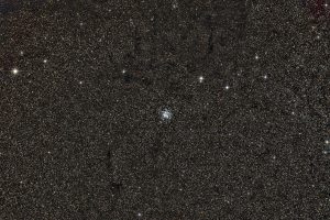
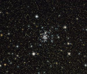
Finally, Figure 16 shows the open cluster M11 in the magnificent Scutum star cloud. Again, this is a total integration time of around nine hours using 10-minute sub-exposures.
MiniWASP Parallel Imaging Telescope Array 2.0
So, I guess that’s it then? We have finally come to the end of the road with all the permutations and combinations possible? Nope. I still wanted a bigger field of view than that offered by the Sky 90/M26C combination – twice as big if possible. Problem is, where do I find a telescope with half the focal length of the 405-mm Sky 90? Well, not with a telescope, but there are plenty of high-quality DSLR lenses around at that focal length, and shorter.
However, having used them in the past, I have found there is a potential serious issue with DSLR lenses. I found that you can get terrible star shapes at the outer edges of the FOV when using DSLR lenses, especially zoom lenses. Looking up the current situation on the Internet, I discovered that the Canon 200-mm f/2.8 Prime lens, stopped down to f/4, apparently gave high-quality results on stars across the whole FOV. This must be worth a punt, so I bought a Canon 200-mm prime lens and put it on a Canon 5D MkII to test it out.
Where do I mount this? Back on the trusty old C11, of course. So, with another kluge bolted onto the back of my poor-old C11, I tried out the Canon 200-mm prime on a Canon 5D MkII DSLR and got the results you can see in Figures 17, 18 and 19. Wow! Well, even with an unmodified Canon 5D MkII, that was way better than I was expecting. These were five-minute subs around one-hour total exposure time at f/4 and ISO 400.
So, the only thing left to do now is put an M26C on the back and see what we get. But before we do that, there are just a few things to change. First, I really don’t like the eight diffraction spikes that we get around bright stars with the Canon 200-mm prime lens stopped down to f/4. That’s an easy one to sort out. I just put a 52-mm UV/IR cut filter over the front of the wide-open lens, which will give me f/3.8 and no diffraction spikes.
I need to fit an autofocuser to the lens, as I don’t have the Live View facility of the Canon 5D MkII, which made focusing very easy. Enter Tom How again who put together a very nice Arduino-driven stepper-motor drive, which turns a toothed belt attached to the 200-mm lens. A little trick to note here, if you want to do this for yourself. When putting the CCD camera onto the back of the DSLR lens, put it 1.0 mm or so closer to the lens than it should be.
Why? So that when you want to take a V-curve for FocusMax autofocusing, you have enough focus travel either side of the infinity focus point. Finally, if I were to only use one 200-mm lens, I would be limited to imaging at f/3.8. The three Sky 90s working together make an effective f/2.6 system, so a single 200-mm lens would effectively “slug” the performance of the array. But if I have two Canon 200-mm lenses working in parallel, then these would give me an effective f/2.7 system, which is close enough to the Sky 90 array performance as makes no difference.
So that’s the final iteration (for now) then for the 200-mm lenses on top of the array. Two of them, in parallel, each working at f/3.8 with a front circular aperture, and each autofocused using FocusMax and a stepper-motor belt drive, with the lens assemblies fitted to the top plate of the MiniWASP Parallel Imaging Array. In Figures 20, 21, 22 and 23 you get an idea of what the lens array delivers.
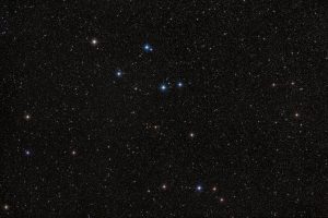
Figure 20 (Castor and Pollux) is a horizontal two-frame mosaic with the Canon 200-mm lenses. Take a look at the sky next time Gemini is there and see just how big a field of view this kit covers. Finally, I have gotten the size of FOV I want to capture.
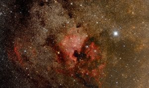
Figure 21 is a horizontal three-frame mosaic of the North America nebula region. Each frame is around four-hours’ worth of 20-minute sub exposures. Good point: huge FOV. Bad point: a “soft” looking image, because we are working at six arc-seconds per pixel. OK, so you can’t have it all ways; I’ll just have to live with that.
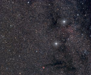
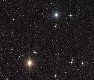
Figure 22 shows an image that I had wanted to capture for more than five years before finally nailing it. This is the “Beehive” cluster, M44, contained within four bright Cancer stars acting as a “Stargate.” This is again a horizontal two-frame mosaic, as I wanted to capture the two bright red Carbon stars that can be seen on the lower left-hand side of the image.
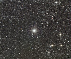
Finally, Figure 23 shows the bright star Caph in Cassiopeia in another horizontal two-frame mosaic. I use the M26C CCD in “portrait” mode, so that by taking two horizontal frames, I got a more square-looking image, which I find more pleasing to the eye.
All that glass in the Canon 200-mm prime lenses does mean that you get bad ghost flaring, but only from the brightest stars, typically those of magnitude less than three. So, the 200-mm lens array is not ideal for those single bright star shots – the Sky 90s remain supreme there.
I did not design the array to have a pair of DSLR lenses sitting on the top of the frame, so dome aperture restrictions mean I cannot run both the Canon lenses and the Sky 90s at the same time, which is a great shame. If I had bought the larger Pulsar optical dome (as I had intended to) at the beginning, then I could be using both systems together. Live and learn, I suppose.
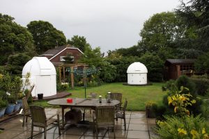
So, there we have it. Figure 24 shows the twin domes at the New Forest Observatory. This is the current state of operation at the New Forest Observatories, Hampshire, U.K. I don’t pretend for a second that this is the end of the story. Look at that lawn – must be room for another three observatories at least. Clear skies!

By Greg Parker, Emeritus Professor of Photonics
Greg Parker is Emeritus Professor of the University of Southampton where he was Professor of Photonics in the School of Electronics and Computer Science. Greg lives in the New Forest (U.K.) with his wife, son, dog, cat, Koi, Celestron Nexstar 11 computer- controlled telescope, and Toshiba Libretto U100 – “the most portable/useful sub notebook – ever.” He has recently finished constructing his retirement project – the “mini-WASP” imaging array at the New Forest Observatory – which is now one of the most powerful amateur astro imaging facilities on the planet.
Editors Note: To show the images in greater detail they are included here.